Protection in Excel

Excel Protection

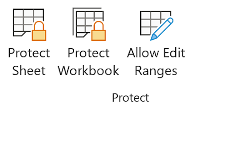
Did you know that in any new Excel file, all cells are locked? However, this locking doesn’t take effect until the worksheet is protected. To protect a worksheet, you visit the Review tab of the ribbon, then toward the right section, you see:

Let’s see what happens when you simply select Protect Sheet. You’re presented with this dialog:

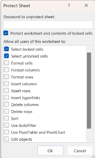
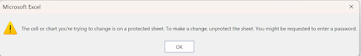
There are many choices in this dialog, and you can scroll down for more (which we’ll look at in a bit). With the above choices of allowing you to select both locked and unlocked cells, you don’t see much of a difference until you try to type in any cell:

Before you protect the worksheet, you should unlock all the cells that are allowed to be changed. For example, in a worksheet in which you have to fill in information, like in this simple illustration:

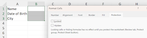
You select all the cells which will contain data and unlock them. Pressing Ctrl/1 brings up the Format Cells dialog, then you select the Protection tab and deselect the Locked checkbox. When you next protect the worksheet, the user can only type in cells B1:B3.

To make it easier for the user, you should probably uncheck “Select Locked Cells” in the protect sheet dialog: 

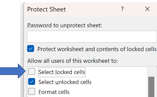
In this way, the user can only click where he can enter data.

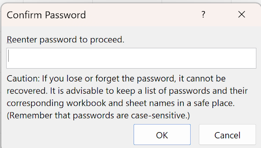
Anyone can unprotect the worksheet and all your settings are ignored, but you can prevent this by using the password. You can enter anything at all for a password, but you must remember it! Once you enter a password, you will be prompted to re-enter it, for safety. Here’s the re-enter dialog: 

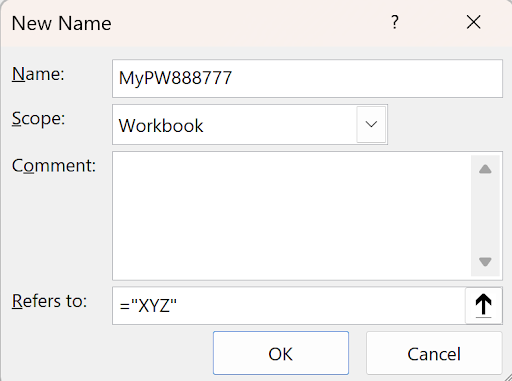
Here’s a suggestion to know you won’t forget a password, but nobody else will be able to discern it. Define a name in every workbook you create that will be password protected. Say that’s MyPW. Or maybe something more cryptic, like MyPW888777, or something you will remember. This name will contain the password, like this:

Anyone can see this, but you can hide names! In the immediate window of VBA (Ctrl/G from within the VBA window), you can do this:

Names("Mypw888777").Visible=False

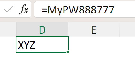
Now it won’t show up in the defined names list or in the Name box dropdown, but you can enter it anywhere to see the password:

It was mentioned earlier that when you protect a worksheet, there are more choices for what features are available or not. Here is the bottom of that expanded list:

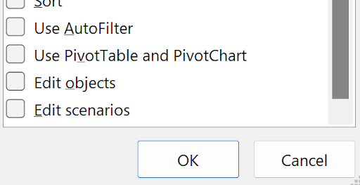
As you can see, there’s only one new item, Edit scenarios. (It seems to this author that Microsoft could have included this last line in the original list!)

When you check any items in the list, you allow these features to be available even if the sheet is protected.

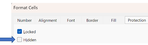
In general, all formulas should be protected. You might have also noticed a checkbox called “Hidden” in the Format Cells dialog – repeated here for convenience:

When a cell is marked as hidden and the sheet is protected, you won’t see the cell’s contents or formula when you select that cell. Here’s a cell that contains =1+1 and marked as hidden:

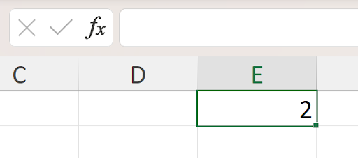
The result shows, but not what’s in the cell!

Protecting a workbook is different from protecting a worksheet. When you use this command, you’ll see:

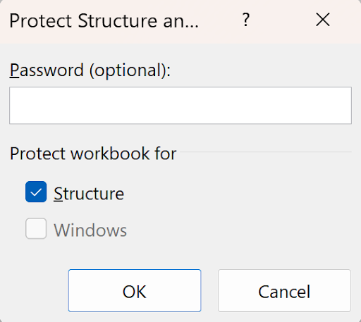
It’s your choice again to use a password or not, but the only checkbox which you can select is “Structure.” The one for Windows is from earlier versions of Excel and is no longer used. When you protect the structure, you can’t add or delete worksheets, nor can you rename, hide, etc. a worksheet. You can see from the right-click of a tab that many commands are disabled:

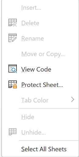
You might do this if, for example, you have VBA code that needs to ensure that a particular sheet is named in a particular way so that there’s no macro error should a user change the tab name.