Functions Built to Work with a Database

Functions Built to Work with a Database

Many of Excel’s functions work anywhere – with any cells’ contents – regardless of the way the worksheet is laid out or where the cells referenced in the function are, relative to each other. All you typically need to do is supply the right values (numbers or cell addresses versus text, for example) for each argument in the function, and the result is accurate. 

Not so with the D-versions (D for Database) of some of those same functions. AVERAGE and DAVERAGE, for example, still total a series of numbers and then divide that total by the number of numbers in that total. But for the DAVERAGE, the numbers can’t be all over the place, they need to be in one field (column) in the database, and that field needs to be referenced very specifically in the function. For a plain old AVERAGE, the numbers you include can be anywhere, and all you need to do is hold down the CTRL key as you click on all the cells you want to average. DAVERAGE is more strict about where the averaged numbers are because it’s doing a simultaneous lookup for the field you’re asking to average and doing the average calculation at the same time. 

So, the D-version relies heavily on where the values are in relation to each other, and the layout of the worksheet is crucial. What does that mean for you? It means you have the ability to perform calculations based on data you’ve stored – purposely – as a database. So, you can refer to your data by field names or numbered columns, and make instant changes in the result of your function, just by typing a new field name or changing the criteria for that field. It’s a level of automation that the non-D-version simply can’t offer. And for each of the D-version functions I’ll cover in this article, we’ll demonstrate just that!

Wait. What Exactly Do We Mean by “a Database”? 

Good question, and something important to clarify from the start. Database nerds, please bear with me – not everyone reading this is steeped in fields and records every day, so we need to set the foundation. 

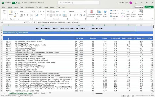
A database is a series of rows (records) and columns (the fields, or pieces of those records) that contain information you want to store, sort, filter, and otherwise use to track values, chart your progress, and make decisions. It could be a list of all of your customers, your products, your transactions, or values stored about the outcomes of medical treatments, student test scores, a farmer’s crop yields, or rows and rows of weather data. Like I said, a database can be set up to store virtually any kind of information. Here’s the data we’ll be using in this article, a database of foods organized by type/group, with each item’s nutritional values in a series of separate fields. 

And What About Tables? 

For users of Microsoft Access – and other database applications – data is stored in what are known as tables, which is just another word for a block of rows and columns. In recent versions of Excel, however, the ability to formally classify a range of rows and columns as a table has been added, and you can apply database functions to those designated tables. But you don’t have to. Your data can remain in a simple range or block of cells, and it will work just fine, allowing you to sort, filter, and use database functions to fully analyze that data.

And, for the purposes of the D-versions of the functions we’ll cover in this article, the data will not be converted to a table. But, if your data is already set up as an Excel table, you can still do everything I’m doing in the instructions and videos in this article. You can also check out Excel’s Table tools if you want to. The bottom line? 

All that needs to be in place for these functions to work is:

• A range of cells containing your data, with no blank rows or columns within it (blank cells are fine)
• A row of field names directly above the first row of the aforementioned cells
• A range of cells, separate from the database range, designated for the values required by the D-Function’s arguments: Database, Field, and Criteria (this range is known as the arguments range)

And that’s it. That’s all that you need to use database functions, so you’re probably good to go. And if you don’t have a database to work with yet? You can download mine to play with, by clicking here:

https://docs.google.com/spreadsheets/d/1ZBekyZMHUHt6gQI0grHVd-MfSjSNlfTL/edit?usp=sharing&ouid=109458182170120820541&rtpof=true&sd=true

So back to the database setup. Most people place the aforementioned arguments range above their database title and field names, so all of that might start on row 6 or 7, with your title row (“Names & Addresses,” for example) and then below that, your fields (First Name, Last Name, Address, City, State, Zip, etc…), and then your records. Shown here, providing the arguments range above the database makes it easy to edit that range and see the criteria, the results of your function, and the database all in one place. 

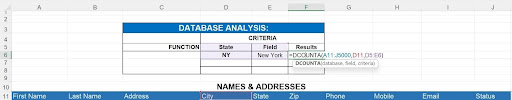
The argument range in the image here, which contains a DCOUNTA function, would allow you to count the number of people living in New York, NY. The State field is used to confine the count to just those records with “NY” as the state, and as cell D11 fulfills the “field” argument, people who live in Buffalo, NY are not included – just people in the city of New York.

TIP - Did you find all that table talk intriguing? Turn your database into a table by clicking within the data and then going to the Insert tab and clicking the Table button. This, after confirming the range of cells containing your data, converts your data to a table. To reverse the process? Click Convert to Range on the Table Design tab.Either way, you can use all of the D-version functions in this article. 

Want to learn much, much more about storing your lists in Excel – and converting them to tables? Check out this in-depth video:

https://drive.google.com/file/d/1vRZRz9nfJC4TdvBImSCr7Lvqe5wjk-De/view?usp=sharing

Setting Up Your Arguments Range

The first thing you want to do for a database that you want to analyze using the D-versions of the functions we’ll cover here is to build the range that I like to call the “Argument Range.” I call it that because it’s where we store the values for the three (3) arguments that every D-version function requires:

• Database – the range of cells containing your field names and rows of records
• Field – the field name for the data you want to use for the purposes of your function
• Criteria – the variable or condition/s you want Excel to consider in performing your function

Shown here, the setup is pretty simple, you just need to create a space for the cells that will contain the values for those three (3) arguments. Using the foods database, we’re asking to average the calories for all the Snacks that have more than 50 calories. So the function (DAVERAGE, in cell E4) is citing the 4th column in the database (which is Calories), and in cells D3 and D4, we specify we only want Snacks and in cells C3 and C4, we’re setting the value to look for in the Calorie field.

It’s essential that the field names and field values (Calories, >50) are set up as shown – the field in one cell and directly in the cell below that, the value to look for in that field. You can have as many of these pairs as you want, in columns across the argument range, and just drag through them when satisfying the Criteria argument in the function. In the sample shown, the range of C3:D4 includes the Calories and Food Group field’s criteria. 

TIP - You can have as many columns as you want, in addition to the one I’m showing in the image for Calories. I could also have a pair of cells for the Protein field, and/or one for Carbohydrates, and enter ranges into the cells beneath the field names. I can also enter a specific value below the field name. So, thinking of a Names & Addresses database, you could have a Last Name, City, and State column, each with a value to look for beneath them – as in Smith, Philadelphia, PA – in that order. Then only the people with that last name, living in that city. And in that state would be the records used in my database function. 

With your Argument Range set up above your database, it’s time to dig in and start using the D-versions of the 12 data analysis functions we’re covering here. Ready? Set? Go!

D-Functions, One by One

In this article we’re going to look at 12 different database-only functions:

• DSUM
• DAVERAGE
• DCOUNT
• DCOUNTA
• DGET
• DMAX
• DMIN
• DPRODUCT
• DSTDEV
• DSTDEVP
• DVAR
• DVARP

All of them, as their names imply, are variations on a single, non-database function. For example, DCOUNTA is a variation on COUNTA, and DPRODUCT is a variation on PRODUCT. These functions work just like their non-D versions, but the twist of adding a database to the mix and setting up criteria pairs of field names and field values is what makes them powerful. And hopefully interesting! 

D-Basics: DSUM and DAVERAGE

Obtaining a sum or average of the numbers within any field in your database could be achieved simply by inserting the standard SUM or AVERAGE function at the foot of that field – in the row below the last value in that column – whether there were 10, 100, or 10,000 records in the database. In, fact when a database range has been converted to a table, you can click in that cell at the foot of any field and choose from a series of common functions to do just that. 

But because databases contain various types of records – customers who are active or inactive, products that are in stock or discontinued, students who are majoring in different fields of study – a DSUM or DAVERAGE is what you need to calculate those values based on those classifications. 

As I’ve said, all D-version functions require the same arguments – the range that represents the entirety of the database, the field you want summed or averaged, and the criteria, being the value (or values) by which your records would be grouped to get the number you seek. So, thinking of the student database example, you could say you want to SUM the number of classes taken by students majoring only in Political Science, or AVERAGE the test scores of students assigned to a particular student advisor. 

Now here’s the cool part. Once you’ve completed the sum and/or average, all you need to do to see (in this case) the total calories or average protein levels for different food group is change the value typed into the Criteria range (under the Food Group field heading). So, to see the total calories or average protein for the Beverages food group, I simply change Snacks to Beverages in cells D4 (for the sum) and D5 (for the average). 

Counting in a Database with DCOUNT and DCOUNTA

Assuming you’re reading this article serially, you just read about using the very simple functions, SUM and AVERAGE, in their D- or database versions. That coverage should put you in good stead to create DCOUNT and DCOUNTA functions. 

If not, if you zeroed in on this section specifically to learn about counting records using a database function, below are the steps you’ll need. Bear in mind that the COUNT function (as well as DCOUNT) counts cells containing numbers, so the field you choose should be one that contains number values, rather than text. 

1. In the argument range above your database, follow these steps:

1. Click in the cell that should contain the DCOUNT or DCOUNTA function.

1. Type =DCOUNT (or DCOUNTA) and press TAB to insert the opening parentheses. 

1. Enter the first argument – the range that makes your database – by clicking in the cell containing your first field name, and then press the CTRL + SHIFT keys. With those two keys pressed, tap the right arrow key (to gather all of your columns) and then the down arrow key (to gather all of your rows). Release the keys.

1. Type a comma, and then enter the number of the field you want to count. Starting with the first column, count across and the number of the column containing that field is the number to enter. 

1. Type another comma, and drag through the cells containing the criteria for your counting. For example, if we’re counting the number of Snacks in our database, select the cell into which you previously typed that field name. 

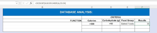
So, in the example, we’ve discovered that there are 30 Baked Foods with more than 500 calories and also more than 50 grams of carbohydrates. We’ve used column 6, Protein, to further verify that none of the records meeting that criteria are missing their Protein value. 

Hey – What About DCOUNTA?

DCOUNTA works the same way, except that it counts non-blank cells – and it works in fields containing text or numeric values. This allows you to count any number of records based on any criteria – not just based on fields containing numbers. So in the food and nutrition database, I can count how many Baby Foods have a certain level of protein or how many Beverages are high in sugar, but I can also count how many foods overall contain the word “beef” or have a “Snack” designation as their Food Group.

Finding a Very Specific Value with DGET

The DGET function is extremely handy for finding one specific value in a particular field. Obviously, this is also even handier with a really big database, where you can’t simply scroll through and spot the value by eye. And, it’s better than the Find tool (found on the Home tab), because it looks in just one field and only in your database range. 

To use this function, you’ll supply the same three arguments (database, field, and criteria), but the criteria is the value to look for in the field – it won’t be counted or averaged in terms of how often it appears, it will be returned, matching whatever you typed in the Criteria cell. That’s if the value is in fact found in the field you’ve chosen. 

TIP - The DGET function either gives you the result you seek, or, if no record matches the criteria, you’ll receive a #VALUE! error. On the other hand, if more than one record matches the criteria, you’ll see a #NUM! error appear as the result. These aren’t technically errors, in that simply indicate the presence (in quantity) or not of the value you seek. 

To look for a different value, just type a new value in the Criteria cell – perhaps correcting spelling or eliminating unwanted spaces in that cell if you received the aforementioned #VALUE! error, indicating Excel couldn’t find what you were looking for. 

Take the High Road (or the Low Road) with DMAX and DMIN

What was the highest test score received in the Biology 101 final exam? Which widget from Vendor A has the highest cost? Use DMAX to find out. Conversely, the lowest score on the same exam would be revealed by the DMIN function, as would the lowest price for a widget from Vendor A. 

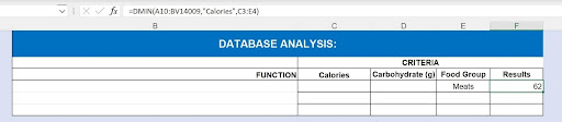
Using my food and nutrition database, to find out how many calories are in the highest-calorie Beverage, I would use the following DMAX function:

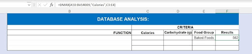
As shown, the function itself tells Excel what to look for (the highest value) and the column number says to look at the Food Group field when viewing the Calorie values, which I indicate in my entry for the Criteria argument. 

To find out how few calories are in the lowest-calorie food from the Meats Food Group, I’d use the following DMIN function:

Multiplication with DPRODUCT

DPRODUCT is based on the PRODUCT function, which exists only to multiply values in cells specified as the arguments in the function. That’s really it – multiply this cell by that cell and put the result here. 

In the D-version PRODUCT, DPRODUCT, Excel will go a bit deeper, and multiply values found by the function and have them appear as the function’s result. 

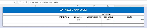
Shown here, the DPRODUCT function calculates total protein all Meats with more than 250 Calories per serving.

Again, the beauty of using DPRODUCT for this result is that by simply changing the field and criteria, you can instantly get a result for any value in the database, for any group of records, based on any standard. So changing Meats to Snacks would give you a new result, for that Food Group.

Calculating Standard Deviations with DSTDEV and DSTDEVP

Using the DSTDEV function (and DSTDEVP) requires first understanding what the term standard deviation means. 

A standard deviation calculation tells you how spread out your data is – how far the values in a given field spread out across a spectrum of values with the mean at its center. Here’s a visual to help you see what I, um, mean:

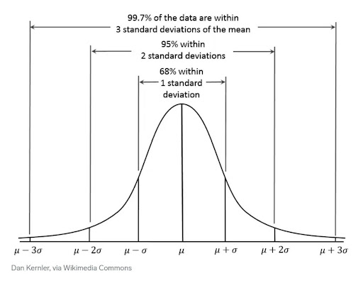
TIP - Wait – what’s the mean mean? The term mean, or arithmetic mean, to be exact, is just another word for the average. It is the sum of all the values in a range of cells, divided by the number of values on the list. To find the mean, add up all the values in a range of cells, and then divide that total by the number of values included.

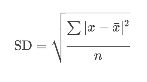
Now, for those of you who can do serious math, here’s the actual formula that’s going on behind the scenes when Excel is performing the DSTDEV function – as you can see, it’s not something the average person can whip up on their calculator or build from scratch with ease.

Using our food and nutrition worksheet, we can calculate the standard deviation for one of our food groups – using any of the fields we might be interested in for analysis purposes. For demonstration, I’ll use the Calories and Carbohydrates fields with only records designated as Baked Goods in the Food Group field to distill the list of foods to analyze in terms of their protein levels. 

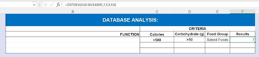
So, as shown, there is a standard deviation of 7 across the Protein values for the foods that meet my criteria of being a Baked Food with more than 500 calories and more than 50 grams of carbohydrates.

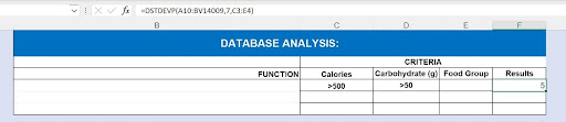
But what about DSTDEVP? 

The DSTDEVP function works the same way, but takes the entire population into account – and by population, I mean the entirety of the field you choose to analyze. It’s a broader evaluation you can use when you don’t want to isolate just one group of records within a database. Here’s the DSTDEVP for the same data but for all of the foods groups in the database, and we see that without confining the records to high calorie, high carb foods, there is only a standard deviation of 5 for protein levels across the whole database. 

Determine the Variance Across Your Data with DVAR and DVARP

Many people – understandably – confuse the concepts of standard deviation and variance. And you may still be confused after this, because I’ve looked out at glazed eyes after issuing the following explanation in classrooms many, many times:

“Standard deviation measures how far apart numbers are in a data set. Variance, on the other hand, gives an actual value to how much the numbers in a data set vary from the mean.”

So, to simplify even further, standard deviation is how much spread you’d see between all the values in a given field, measured against that mean, or average value. Kind of like seeing the MAX and MIN values along with that AVERAGE, all at once. Variance measures the difference between the numbers – cumulatively – along that spectrum from the lowest to the highest, with the mean in the middle. 

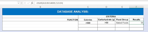
Using the same subset of data again, we’ll calculate the Variance for the Protein values for a group of foods – using the same three arguments all D-version functions: Database, Field, and Criteria. Here’s the function in place, showing I used the same Criteria for Calories and Carbohydrates, and the same Food Group.

It’s Fun to Say DVARP

And like DSTDEVP calculates the standard deviation for an entire field, so the DVARP function calculates the variance across an entire field, rather than from a selected group of records’ values within that field, so in this case, it would ignore the Food Group value in the Criteria range and show the Variance across all foods in the database.

Wrapping Up

So, that’s a wrap! Your Excel database analysis tools just increased by 12! You can also check out these videos for more info on other powerful Excel database features:

Reorganize and Analyze with Pivot Tables

Use Pivot Tables to organize the fields you care most about in a way you can use to see key information in the layout that makes the most sense to you. These three videos will give you a jump-start:

Creating a Quick PivotTable (https://drive.google.com/drive/folders/1XIat75PY9RS0S8BB3ikyh0lqIVZAgSIs?usp=sharing)

Understanding PivotTable Structure

https://drive.google.com/drive/folders/1RqbCcX9hx75l0_yc8Ew7vViImXqmmmTS?usp=sharing

Editing a PivotTable

https://drive.google.com/drive/folders/1a7XFzLgnha_6hiiQV6YHCy4Vw-D8ms4T?usp=sharing

Find it Fast with XLOOKUP

The new version of VLOOKUP and HLOOKUP, XLOOKUP is designed for working with database ranges and tables to quickly find the exact record or records you need. Use the XLOOKUP function to build interactive forms where people enter just one piece of information and receive essential fields’ data instantly – and get started with this powerful function here:

Finding Data with XLOOKUP

https://drive.google.com/drive/folders/1KmEuKFtWc0E4vQFIuZZZkvP_7fvByDOu?usp=sharing