Formatting Cells in Excel

Formatting Cells

Excel has many ways to format a cell. In prior articles, Cell Styles were discussed, as well as Number Formatting. In this article we’ll discuss other kinds of formatting, including borders, colors, alignment, font, size, underlining, orientation, and others. 

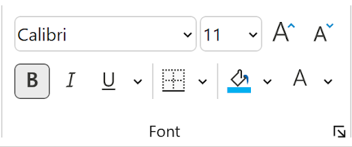
These options are all covered in the Home tab. Let’s first look at the Font group:

The Font dropdown has many fonts to choose from. For example, here’s just the beginning of that list:

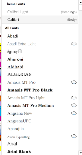
As you can see, many of the fonts have an icon on the right side, representing the cloud – these are fonts which are not on your system yet, but you can download them from the cloud:

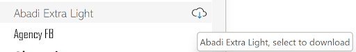
Here, the cursor was hovering over the cloud system and you can see from the tooltip that you can select the cloud to download the font “Abade Extra Light.”

The font size, is the dropdown to the right of the font name, and the listed sizes are not the only sizes available – you can type in a size you want! Here, 31 was entered as the desired size:

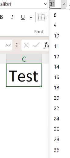
If a cell contains data, then as you scroll down the dropdowns for either font name or size, you see a “live preview” of what the cell would look like if you selected that item.

Underneath the Font Name dropdown are 3 icons for Bold, Italic, and Underline:

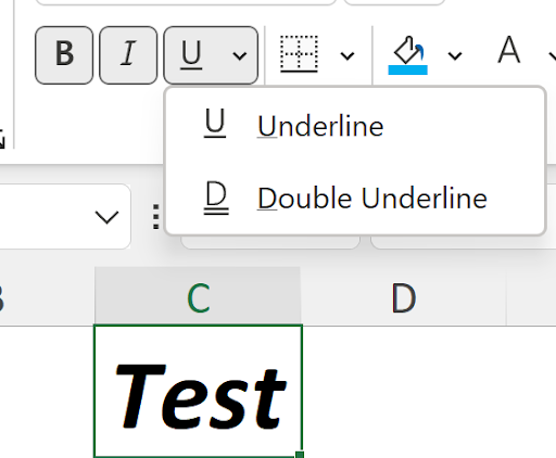
In the above illustration, the word “Test” was formatted as both bold and Italic – these are either on or off. The Underling seems to imply you can underline with either single or double underlining, but in fact, there are other options which you can see by pressing ctrl/1 and selecting the Font tab. In the underline section, there are 5 choices, not just Underline or Double underline. 

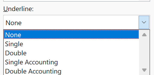
Single, in this dropdown, is the same as Underline in the ribbon choice. But what’s Single/Double Accounting?

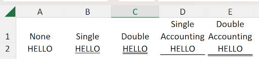
You can see all the choices here:

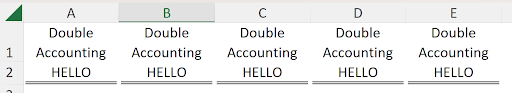
The accounting versions give an underline just shy of the entire width of the cell, not just the words in the cell. You can see here, the small gaps:

To color a cell you can choose between the cell color of the font color. Here’s the difference:

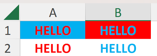
The font color in A1 and A2 are the same (red), and also the same in B1 and B2 (light blue). The cell color in A1 is light blue and in B1 is red. If you make the font and cell color the same, the text is invisible:

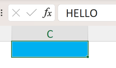
You can see the word exists in the formula bar but can’t be seen in the cell!

When you right-click a cell, you see a “mini toolbar” as well as other commands. The mini toolbar looks like this:

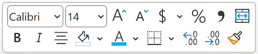
In addition to the ones in the Font group, there are some from other groups, like the alignment and Number groups. Also, the format painter (lower right corner) is included.

Let’s explore the Format Painter - . This is a shortcut for copy/paste special/Formats.

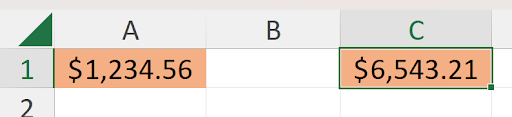
Suppose I want to use the same formatting you see in cell A1 on cell C1:

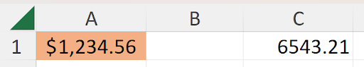
You click A1, click the format painter icon (From the Home tab or the mini toolbar), then click cell C1:

When you click the format painter, a little paintbrush icon is attached to the cursor. Once you click the second cell, the icon disappears. If you wanted to use the format from A1 on many cells which are not adjacent, you can doubleclick the icon and it stays alive until you either click it again or press the esc key.

The border icon, has a dropdown which shows many borders. The one shown is the border of the last time you used the command. That is, if you chose All borders, then the icon in the ribbon looks like this:

You can also choose to “draw borders”:

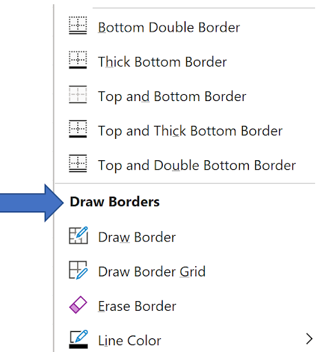
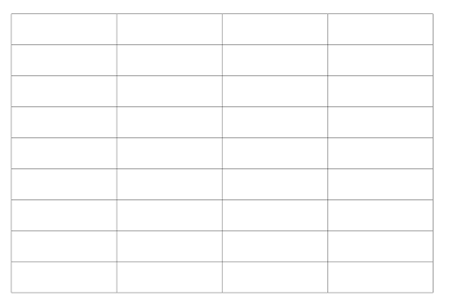
If you select this icon, you then drag the cursor from the upper-left to the lower right of the grid you want to make (you can also select Line Color – the bottom command in the illustration above):

Below Line Color is Line Style (for solid, dashed, etc.) line, and below that is :More Borders, the equivalent of pressing Ctrl/1 and clicking on the Border tab:

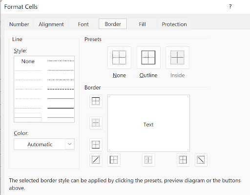
Here, you can also select a color for the border, diagonal lines, etc!

Using the same dialog as above, but with the Fill tab active, you see this:

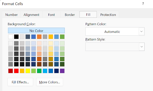
Here, you can fill a cell with any color (clicking “More Colors” gives you access to over 16 million colors!), and you can also click Fill Effects to get this dialog:

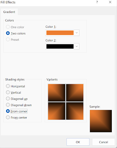
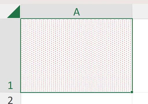
The “Pattern Style” button in the previous dialog brings up this feature:

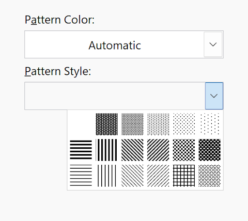
With combinations of the above, your cell(s) can look like this (pretty, fancy, or ugly!)

You can merge cells – make several cells look like one cell. This can make it easy to apply a type of heading over many cells:

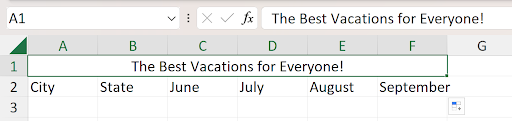
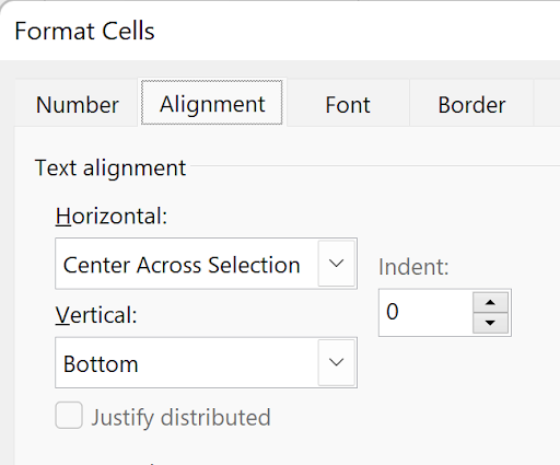
Here, cell A1 spans A1:F1. This can also be accomplished by “Center across Selection” which is in the Alignment tab from Ctrl/1:

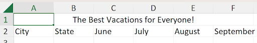
Here, you can see that cell A1 does NOT span A1:F1 – you can tell by the selection border. To get the same effect, you first select A1:F1, then issue the command:

You can see in the previous dialog there’s a feature called “Indent:” – let’s look at how you can use this…

Suppose you have a worksheet something like this:

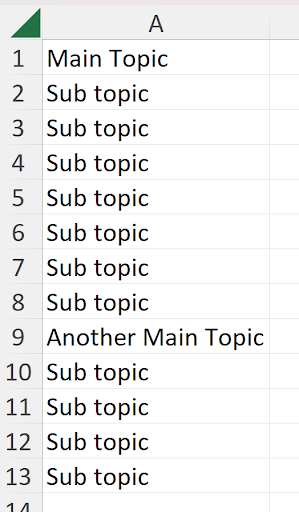
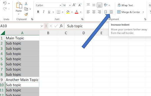
and you want to indent all the sub topics. Many people would select each sub topic cell and type a few spaces in front of each text. But you can select the subtopics (using the ctrl key to select A2:A8 and A10:A13) and then click the indent icons:

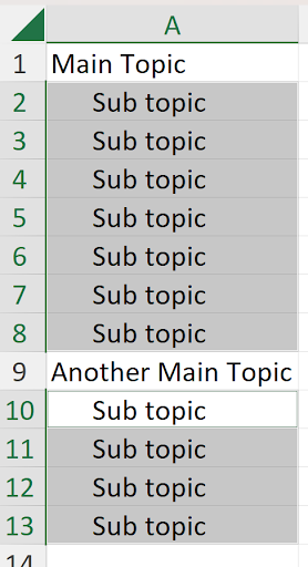
Here’s the result:

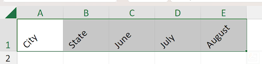
Lastly, you can put your text on an angle! This feature is also in the ribbon:

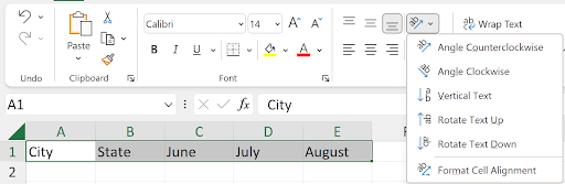
Selecting the first dropdown, “Angle Counterclockwise”, produces this result:

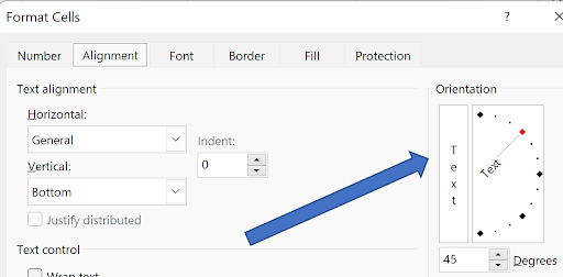
In the alignment tan, you can fine tune this to make it look just as you’d like: