Using Excel's Power Query Editor

Using Excel Power Queries

What’s a Query, Anyway? 

If, like me, you played a lot of the card game “Go Fish!” when you were a kid, you know that the point of the game was to accumulate the most cards. You did so by asking your opponent, “Gimme all your…” and you’d ask for all of their Kings or Aces or 8s, any cards you thought they had. 

So, a query is a lot like asking a database, “Gimme all your…” and then asking for customers with a zero balance, inventory items with more than 50 products in stock, students enrolled in a Level I Yoga class, or contractors with the word “heating” in their company name. You ask a question, and the database gives you the answer, in the form of a list of records that meet your criteria – assuming it has what you asked for. 

In an application like Microsoft Access, queries are a built-in, standard part of the software. You wouldn’t build a database without them, and they can be the basis of data entry/editing forms, reports, and even the source for drop lists and other buttons you can add to forms for greater functionality. Excel, on the other hand, wasn’t designed to be a database application, but has been used as one due to the tabular (columns and rows) structure of its worksheets and the fact that Access isn’t as…accessible to a new user, or so it often seems. So, over time, additional tools for data analysis have been added to Excel, allowing people to make use of the information they’d packed into their worksheets, including tools like the Analyze Data panel, which I covered in another blog post, at this link: 

https://www.nobledesktop.com/learn/excel/excel-data-analysis-with-statistics

Suffice to say, queries in Excel, and certainly Power Query, are – ironically – less “user-friendly” than they are in Access, because they’re an addition to the software, something engineered to add functionality to Excel that didn’t exist before. That said, they’re not too hard to learn or complex to use – but there is a very structured process for building queries in Excel, and that’s what I’ll cover here. 

So, What’s a Power Query?

With Power Query, you can connect to virtually any data source, be it one of your own worksheets or an Access database – or a database created in another database application and stored on a server (which you’ll have to identify by a path to it). 

Once you’ve selected the data source, you can then shape that data, which is Excel’s term for choosing which columns (think fields, to stay in the data mindset) to use and view in the query, how the data will be sorted, and which filters to apply to distill the data down to just the records you want to see. 

You can also combine or merge your query with another query, or combine data sources, or both. In this article, I’ll be sticking with a single data source, and showing you how to make individual queries – otherwise, we’ll end up with a novel that you’d never have time to read. But I will give you links to resources should you wish to go down any of those data rabbit holes on your own! 

After that, you can run your query and save it in a new or existing workbook. Excel calls this loading, but in terms you already are familiar with, it’s just running and saving your query. And by run, I mean execute or perform the query – sort and filter the records and export them to a new location for use and viewing. I have to say that by bringing in new terms for things we’re already familiar with doing, Excel has needlessly complicated this feature. But that’s just one woman’s opinion, you may feel differently. 

So, the four steps in using Power Query are:

1. Connect: Make connections to existing data – in your own computer, on a server, in the cloud, anywhere tabular data can be found. 
2. Transform:  Shape the data to meet your needs, while the original source remains unchanged – by removing unwanted columns (fields) and applying your own sorting and filtering to the remaining fields. 
3. Combine : As desired/needed, connect queries from multiple data sources into a single worksheet.
4. Load: Run your query and load it into a worksheet, where you can view it, use it, and save it. You can also refresh the loaded copy to reflect any changes in the source data.

Building Your Query in Excel

The most important step – taken before you begin the literal process of creating your query – is to plan your query. 

First, determine in which range of cells or table within a worksheet (or external data source, such as an Access table) do you want to make the demand, “Gimme all your…” and see only the records that interest you?

After establishing that, decide what do you want to know. From that table or range, which fields do you want to see, and which ones do you want to use in creating the query? Though Excel never uses the word, you’re going to be establishing query criteria -  the word/s that come after your “Gimme all your…” demand and tell Excel which records you want to see and how Excel should select and display them for you. 

Criteria can include numeric values, dates, or text. So, for example, imagining a database of vendors, you could ask to see all the vendors with whom your company has spent more than $1000 in 2022, but say that you only want to see electricians, plumbers, and HVAC contractors. This kind of query planning will make it much easier to not only choose the right data (that vendors table), but to know which fields you want to filter – the fields that store how much you’ve spent with each vendor, the range of dates you worked with them, and the field that stores the vendor type for each vendor in the table.

It’s important to note that an effective query can include fields in addition to those you use in filtering the data. For example, if you want to contact those vendors who make the cut after you run your query, including the Contact Name, Phone, and Email columns from the table will be handy. 

Connecting to Data

Once you’ve decided which range, table, or database you want to use (and have determined where that data literally resides, as you’ll have to select it now), it’s time to connect. 

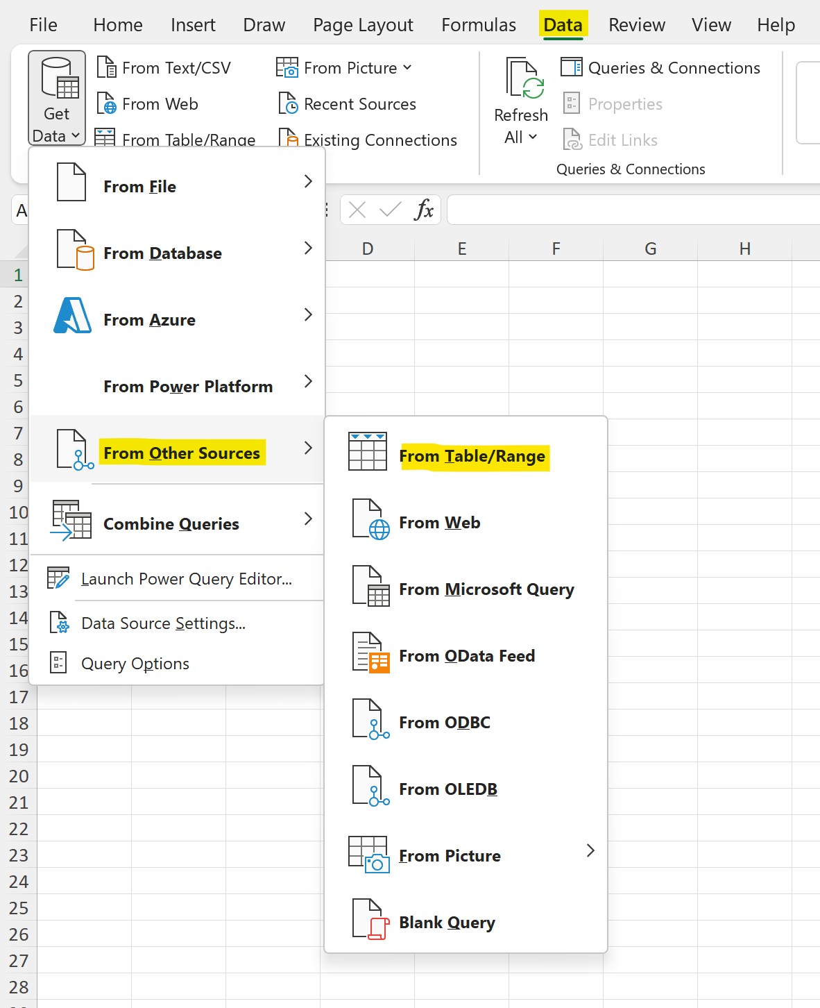
From the Data tab in Excel, click the Get Data button, and then choose From Other Sources. The submenu that appears offers several options, but for this demonstration, we’ll choose From Table/Range, meaning we want to use one of our existing Excel worksheets as the source of our data. 

But What If My Data Isn’t In an Excel Worksheet? 

The process of building a query doesn’t really change after you’ve chosen your source. For the purposes of this article, I’m taking the simplest path and one that most users will need, and our data source will be an Excel worksheet that contains a data range. But if your data isn’t in Excel, just choose the source from that From Other Sources submenu, and then follow the steps from there to identify the location of that data. 

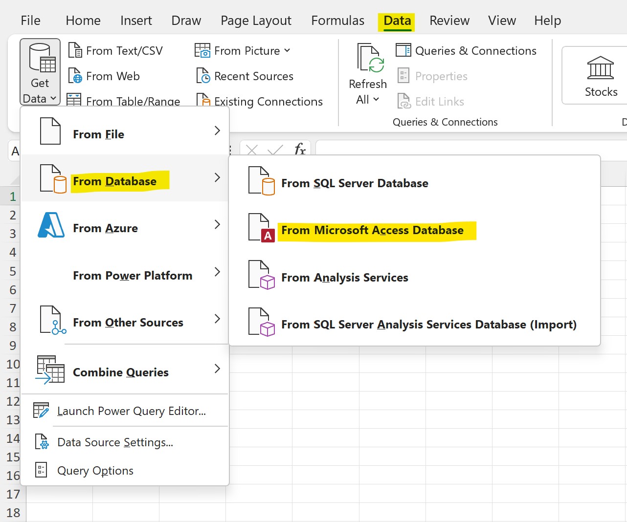
You can also choose From Database, and if you’ve got an Access database – or data stored on an SQL Server – you can choose accordingly from that submenu. 

Whichever source you choose, you have to identify the database and its exact location – on your local hard drive, on your One Drive, on another server, in the cloud – wherever it might be. Sticking to my plan to keep this simple, we’ll continue with the From Table/Range process. 

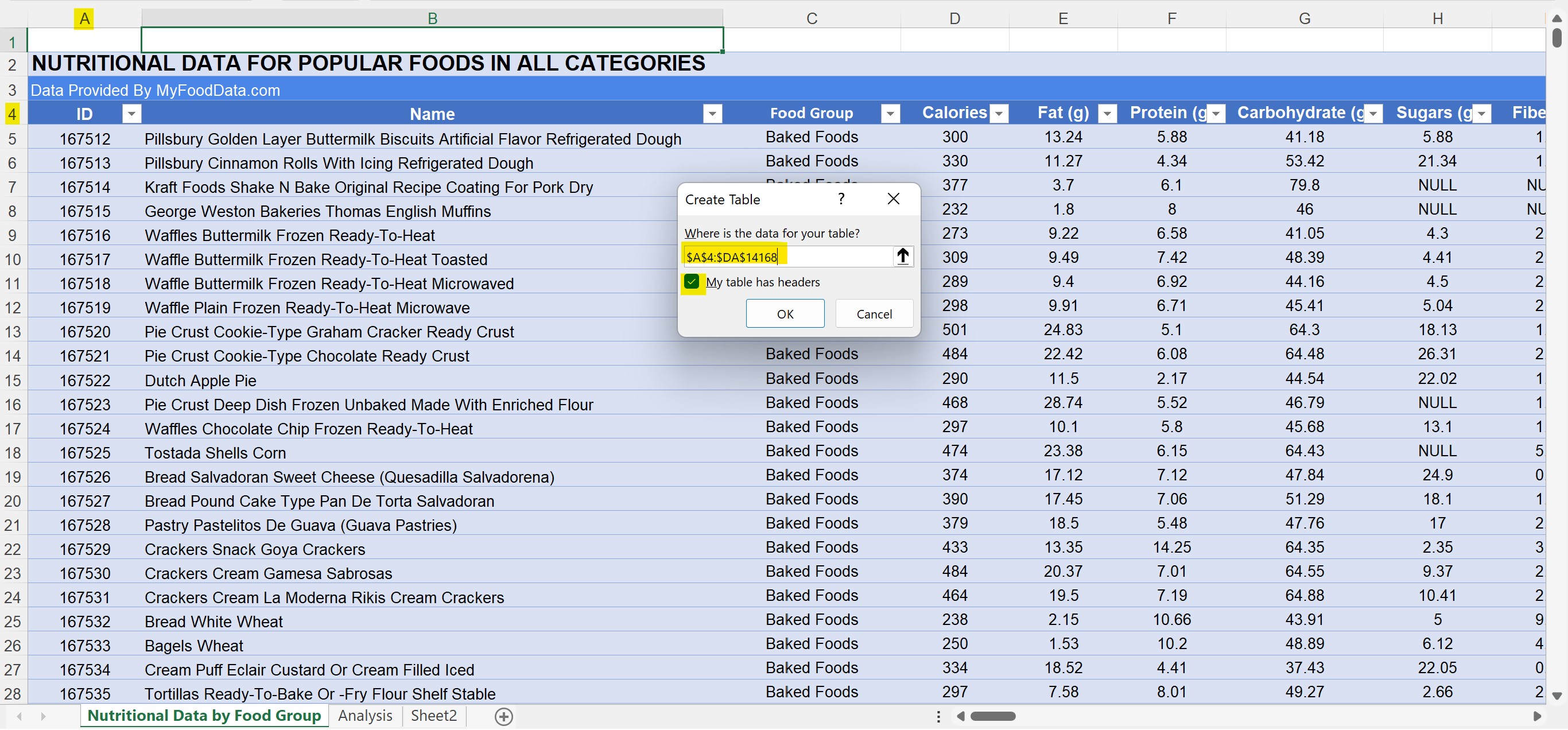
After selecting that submenu item, Excel asks you to identify the table or range you want to use as your data source. As shown here, I have opened the data source first, and Excel wants me to confirm the range of cells that contain both my headers (the field names) and the rows and columns of data. 

Using the CTRL + Shift + arrow keys (with the Right Arrow, to go to the last column, and then with the Down Arrow to go to the last row), I identify my range. My headers (which I’ve indicated I have, so Excel knows to look to the top row for my field names) and my data live in rows A4 through DA14168, which means I have over 14,000 records. 

From here, when you click OK, the Power Query Editor opens, showing Table1 (a name you can replace with something more meaningful) and a series of ribbons, containing tools for choosing the fields (columns) you’ll be working with to query your table for the records (and the fields within them) that you want to see in the query results. 

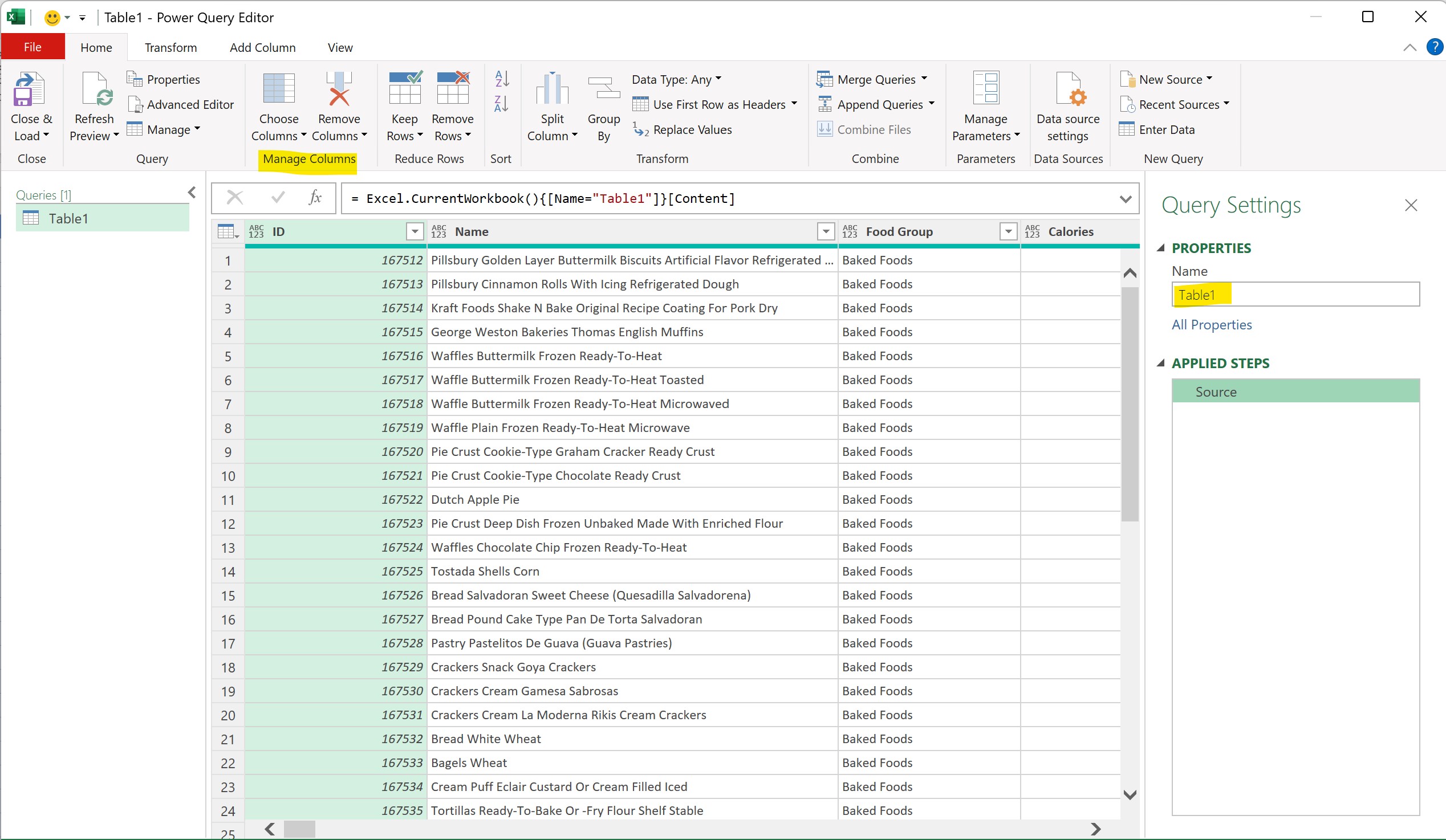
The Power Query window offers five (5) tabs: File, Home, Transform, Add Column, and View. Each ribbon has its own set of tools, just like the ribbons in the main Excel application. Below the ribbons you find what looks like the Formula Bar in Excel, but it’s actually a place for editing the table and fields cited as the source for your query. You never have to interact with this bar, but you’ll see it populate with references to tables and fields as you build your query. 

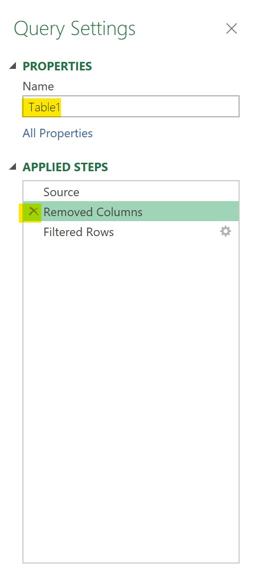
Below that, you have three (3) sections. On the left, a list of queries related to the current table (not in the image here it’s still called Table1, and it’s all alone, as it’s (A) my first query related to this table and (B) it’s not related to any other existing queries. To the right is the Query Settings panel, which gives you a place to rename the query you’re making, and shows a list of the steps you’ve taken thus far in the process. To undo any step, just click the X next to the step and you’re back to the previous step – allowing you to go all the way back to having chosen the table source and nothing beyond that. 

Shaping Your Query

With the Power Query Editor open, your next step is to decide which columns you want to retain – it might be all of them, or if your database has lots of fields, just the ones most important to you – and then to use one or more of them to set your query criteria. Remember, however, you don’t have to remove any of them!

Removing Any Unnecessary Columns from Your Query

If you don’t need or want all of the columns in your table, the first step in setting up the query is column removal, even if it’s just one column. Here’s how to remove the columns you don’t need to see in your query’s results:

Using the CTRL key, click on the header (field name) for the columns you want to remove. You can scroll right and then re-press the CTRL key to continue gathering columns. 

Using the CTRL + click method, gather the columns you want to remove, and then click the Remove Columns button on the Power Query Editor’s Home tab. The two choices that appear are Remove Columns or Remove Other Columns. The latter option will delete all columns except for the ones you’ve selected – so be careful which one you choose!

TIP! If you want to select a series of contiguous columns, press the SHIFT key instead of the CTRL key. With the SHIFT key pressed, click on the first column you want to remove and then click the last column in the series that you want to remove. All of the columns, from the first clicked to the last, are then selected for removal.

TIP! If you make a mistake and Ctrl + click on a column you didn’t mean to select, just keep the Ctrl key pressed and then click the column header for the column you didn’t mean to choose. It goes from selected to un-selected, and you can continue selecting other columns or, if you’re ready, click the Remove Columns button.

Setting Query Criteria 

With the columns you don’t need (if any) removed, now you can use one or more of them to set your query criteria. As I said earlier, Excel calls this shaping the query, but for anyone accustomed to setting up queries in Access or in any other database application, this is simply setting the criteria for your query – the essential “Gimme all your…” settings, so you get just the records you want in the results of your query. 

To set the criteria, use the drop arrow next to the header (field name) for the first column you want to use. Thinking back to the example of querying a Vendors table for certain types of vendors with whom a certain amount of money was spent within a range of dates, these are the fields you’d use, and the criteria you’d set:

Now, in the nutrition database you’ve seen in my examples thus far, I want to see the foods that are grain-based, and see only those with low calories and high protein. So, I’ll set criteria for the Food Group column, Calories, and Protein columns:

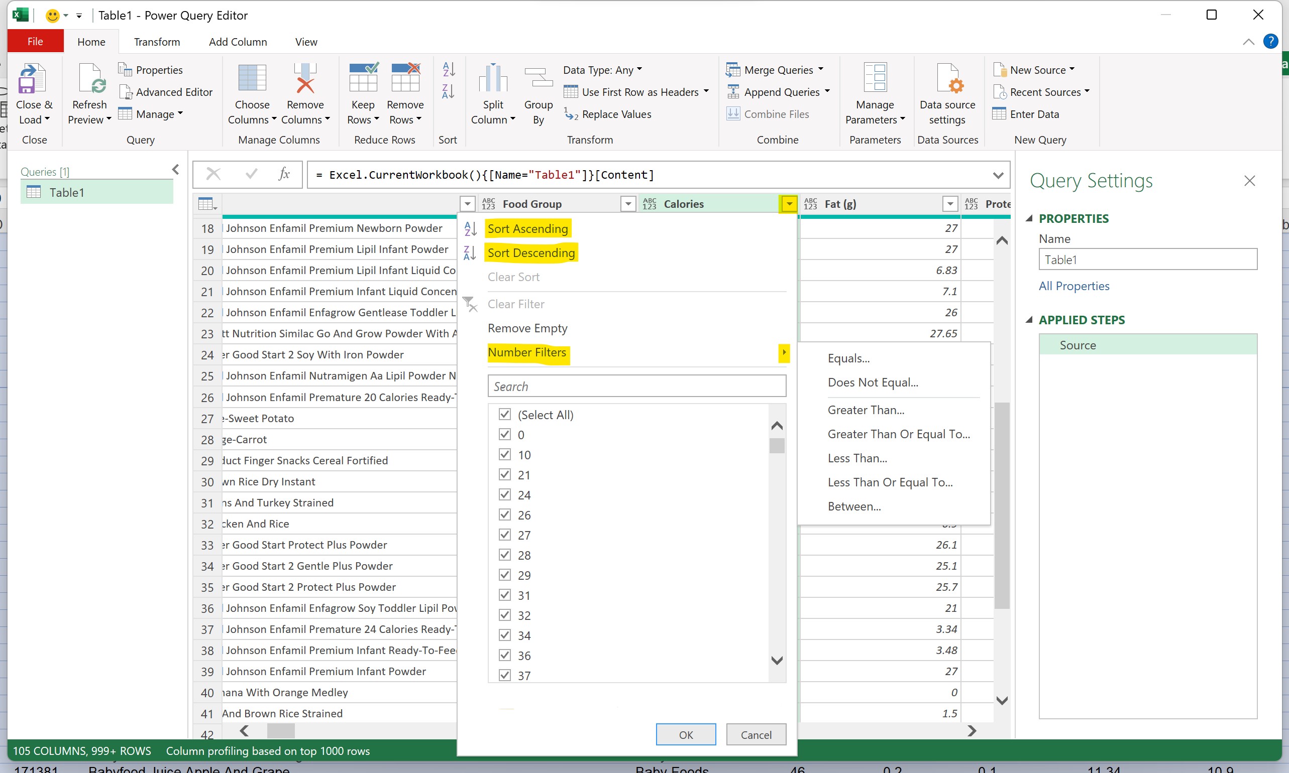
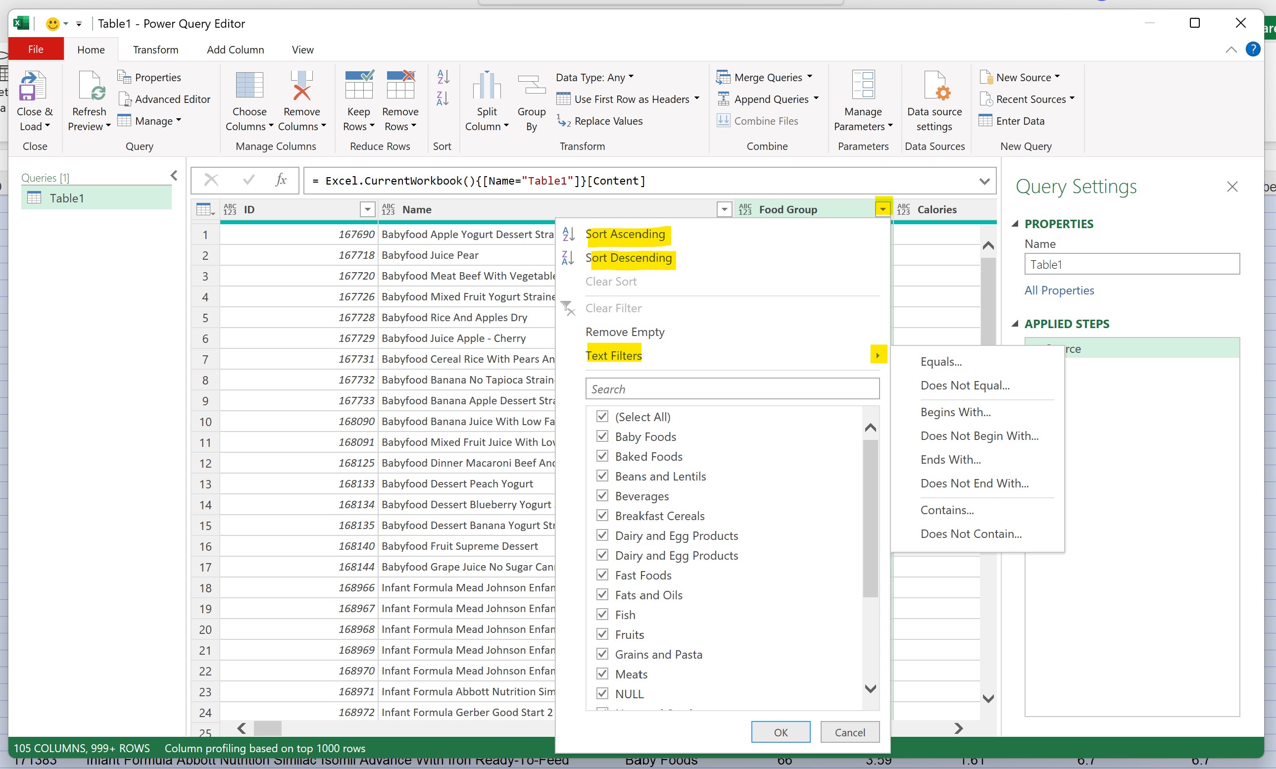
As you click each column’s drop list, you have lots of options – you can sort the records in your database by that given field, you can use checkboxes to choose records by common field values, or you can use filters. The offered filters are determined by the type of data stored in that field, so you’ll see Number Filters in a field containing numbers (including Currency fields), and you’ll see Text filtering options for filtering by the text (characters, words) found in Text fields. 

TIP! Does all this look familiar? It should Excel offers these same sorting and filtering tools for any range that’s been converted to a table. Check out my in-depth videos on sorting and filtering here:

https://drive.google.com/drive/folders/1wzspYb9yaa1Mwl8C56jsrIejAVKicbbB?usp=share_link

https://drive.google.com/drive/folders/1s3updL3dRWdqcTkAa2HaZAUiqh78_Sml?usp=share_link