In this article, we are going to look at how Data Analysis with Statistics can be done efficiently through the use of Microsoft Excel.
Excel Data Analysis: Statistics
I’m just gonna say it. Without statistics, your Excel data would just be a sea of columns and rows, swimming with potentially useless words and numbers.
Why do I say “useless?” Because anyone viewing that data would be hard-pressed to draw any conclusions, understand the information, or take any confident action based on it without some attempt by you to show people what trends, commonalities, and anomalies can be found within the data. These values are known as statistics, and they include:
- simple totals and averages
- the results of more subjective averaging
- percentages
- data comparison values
All of these statistics make your data clearer, more accessible, and best of all, useful.

First Things First: Cleaning up Your Data
Rather than diving right in to the statistical analysis functions I want to share with you, we’re going to start with a series of functions that will help you make sure your data is free from extraneous spaces, are properly formatted for use in calculations, and therefore more useful to your data’s audience.
TRIM Dreaded Spaces from Your Data
The TRIM function lets you get rid of spaces – the enemy of many functions that require criteria to be found within the data to complete their calculations.
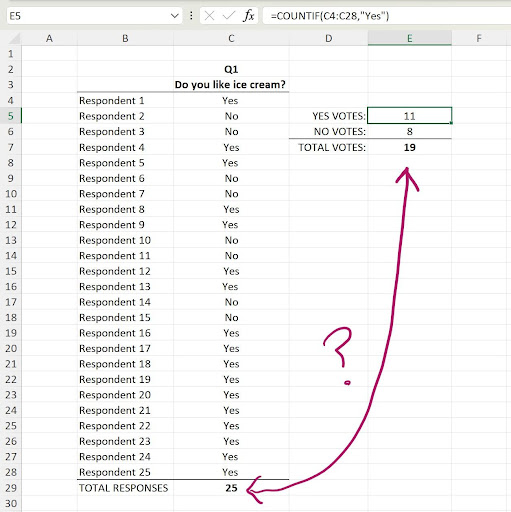
Why are spaces so bad? Well, imagine you’ve set up a COUNTIF function to count how many Yes responses to a survey can be found in a given column. If some of the cells in the column also contain a space – either before or after the word “Yes” – then those responses won’t be counted. Running TRIM on that column will solve the problem.
As shown here, we’ve counted the Yes votes to a question that 25 people answered. The COUNTIF function tells us that 8 people voted Yes, and 11 voted No. But there were 25 responses, and 11 + 8 equals 19. So why were 6 of the votes not counted? Spaces. Looks for “Yes” – note by the placement of the quotation marks, it’s not looking for the word with a space before or after it – the votes entered as Yes_ (with the space typed by the person doing data entry) are not counted. It’s a common mistake, by the way, to type those spaces. We get into the habit of typing a space after every word when we type text into a document, and we forget not to do that when typing words into Excel worksheet cells.
Looks for “Yes” – note by the placement of the quotation marks, it’s not looking for the word with a space before or after it – the votes entered as Yes_ (with the space typed by the person doing data entry) are not counted. It’s a common mistake, by the way, to type those spaces.
We get into the habit of typing a space after every word when we type text into a document, and we forget not to do that when typing words into Excel worksheet cells looks for “Yes” – note by the placement of the quotation marks, it’s not looking for the word with a space before or after it – the votes entered as Yes_ (with the space typed by the person doing data entry) are not counted. It’s a common mistake, by the way, to type those spaces. We get into the habit of typing a space after every word when we type text into a document, and we forget not to do that when typing words into Excel worksheet cells.
Because the Criteria (see the formula bar in the image) looks for “Yes” – note by the placement of the quotation marks, it’s not looking for the word with a space before or after it – the votes entered as Yes_ (with the space typed by the person doing data entry) are not counted. It’s a common mistake, by the way, to type those spaces. We get into the habit of typing a space after every word when we type text into a document, and we forget not to do that when typing words into Excel worksheet cells.
TIP - A very cool thing about TRIM is that it won’t get rid of spaces between words in a cell. So, if the cell currently contains the text, John Smith, it won’t turn it into JohnSmith. It will only get rid of any spaces before or after the entire cell’s contents. What’s another cool thing about the TRIM function? No error results if none of your cells contain extraneous spaces. So, it’s a safe function to run on any data, even if you’ve had no evidence of unwanted spaces so far. Just use it as a safeguard against future issues.
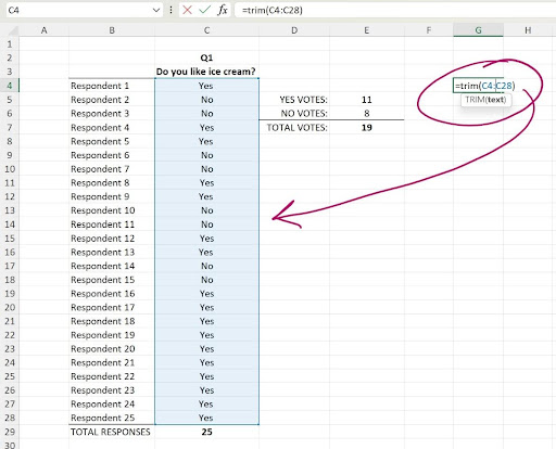
The TRIM function, shown in the formula bar in the adjacent image, has one argument – (text).This argument should be the cell or range of cells you want to rid of spaces. This video demonstrates the entire process, including the replacement of the source data with the data trimmed of spaces.
Converting and Extracting Numbers with VALUE
Moving on from TRIM, which gets rid of spaces to clean up your data, let’s look at another function – or actually a pair of functions – that we can use together to get rid of unwanted content in one column and then move it to another column. Of course, it works in rows, too, but as this is an article about data analysis, and data is typically stored in columns.
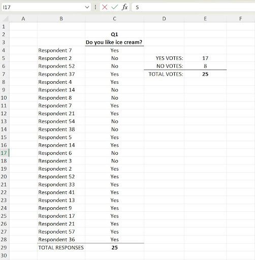 Looking at our votes example again – it’s simple, so you can focus solely on the function/s – let’s extract the voter numbers from cells with the word “Respondent.” After adding a column to house the extracted numbers, I can simply type =VALUE(RIGHT(B4,2)). Breaking this set of nested functions down, we’re asking Excel to extract a number value, found on the right side of the entry in cell B4, and to take just the first 2 characters from the right. If our Voter Number entries had 3 or 4-digit numbers, the RIGHT function would reflect that, as in RIGHT(B4,4).
Combining Cells with CONCATENATE
Now let’s go back the other way! We just used the VALUE and RIGHT functions together to pull numbers out of a string of text, placing them in a separate column. In this example of how to make your data more useful, we’ll put together things that are currently separated.
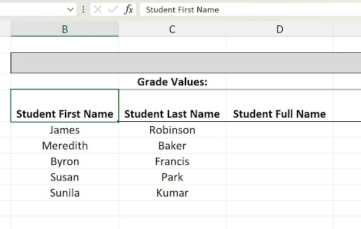
Why would we need to do that? Well, imagine one of the most common types of data we store – names and addresses. We all know the benefit of storing last and first names in separate fields (columns), but what if someone wants to see the person’s full name, in First Name, Last Name order? When you want to combine two or more fields into a single value, with its components separated by spaces, dashes or any symbol you want, it’s CONCATENATE to the rescue.
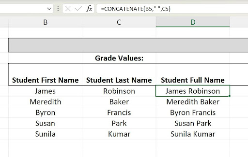 TIP - Did you notice the “ “ inside the function, =CONCATENATE(B5, ” “, C5)? That pair of quotes and a space inserts a space between the two cells’ data, creatingJames Robinson instead ofJamesRobinson. Handy, eh?
Getting Started with Simple Stats
Now that your data is cleaned up, it’s time to generate some useful numbers. Sometimes all it takes is a total at the foot of a column or the end of a row can speak volumes. Or an average can give perspective to your data, helping people to interpret the numbers more realistically. There’s a reason SUM and AVERAGE are the most commonly-used functions by Excel users.
But Wait! There’s More!
If we look at any range of numbers, especially when there are too many to tally in one’s head, a SUM makes all the difference. The SUM enables the viewer to say, “We have almost twice as much income from insurance policies in Michigan than we have from our policies in Maine!”
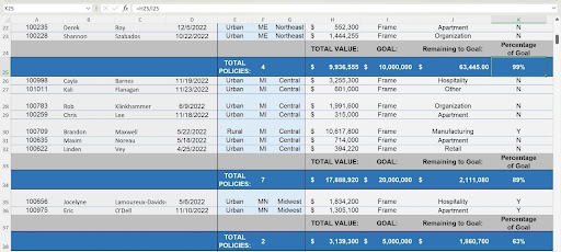
But what’s even more useful? Comparisons. Comparing data is a great way to make it more useful. Knowing the goal, you can compare your SUM to the goal value by subtracting where you are from where you want to be, and you can easily see how you’re progressing.

TIP - Do you have access to last year’s data?Comparing values as of today this year to the same date last year can let you – and your audience – know if you’re on track and compare the performance of products, projects, events, and campaigns. If it’s sales data, registrations, enrollments, or subscribers you’re tracking, knowing if you’re doing as well as or better than last year can tell a valuable story for your marketing and sales people.
Calculating Percentages
I would be willing to bet that there isn’t anyone with a television, smartphone, or a car who can go a single day without seeing or hearing a percentage.
- “Save 20% on your electric bill!”
- “The candidate is leading her opponent by 12% according to the latest polls.”
- “Eating more fruit and vegetables can reduce your risk of disease by 15%!”
- “Wouldn’t you like see your mortgage drop by 5%?”
Here, using the insurance policy data we were just looking at with regard to using SUM and viewing comparative data, is that same data with the addition of a percentage, making it clear how close to (or far from) our goal we are.
Whether informational or inspirational, percentages distill data down to numbers that people can relate to. Saying “8 out of 10 people” is less compelling than saying “80% of people” agree with a particular statement. Going back to the registrations data I referred to earlier, people will love hearing “We’re at 71.4% of goal as of today!” much more than “We just need 143 more registrations to meet our goal!” They’ll want to know exactly how many registrations are still needed, but that percentage drives home that fact that you’re really closing in on the goal.
Calculating percentages is easy. As shown in this video, it’s simply a matter of taking two numbers and dividing them by each other and then changing the format of the resulting number to a Percentage, using the Number Format tools on the Excel ribbon.
AVERAGE Isn’t Always an Insult
Most of us would rather be known as “above average” in terms of our abilities, appearance, income, you name it. But in a database, “average” isn’t a quality, but a quantity. Knowing the average income across all the cities in a particular state or the average age of people who gave a particular answer to a question in a survey are valuable statistics, giving useful perspectives on the data overall, and especially to those particular pieces of the data.
Assuming you know how to do a simple AVERAGE function, we’re going to look at some variations on averaging your data.
TIP - The IF versions of SUM and AVERAGE allow you to specify which cells include in the SUM or AVERAGE, by asking you to supply criteria to look for within your data. =SUMIF(C10:C20, D10:D20, ”>40”) would look in cells C10 through C20 for people whose age is over 40, and then total their incomes in cells D10 through D20. The incomes of people younger than 40 would not be included in the SUM. Make sense? Not sure? Check out this video to find out more:
TIP - SUMIFS and AVERAGEIFS simply allow you to apply multiple sets of criteria to more than one range of cells. This means you can seek sums and averages based on the presence in your data of given words or numbers, found within the data, throughout a database – but without the cells you want to look in having to be in contiguous ranges. These functions provide real power and unleash creative views of your data. Check out this video to learn more:
Taking Averaging to the Next Level
The AVERAGE function is very popular because it puts things in perspective. If your child gets an 80 on their history test, you might be disappointed – until you find out that the class average for that test was 72, in which case, as you always knew, your child is “above average!”
AVERAGE is just the tip of the iceberg, however, when it comes to getting perspective on numeric data.
Weighted Averages with SUMPRODUCT
So, what’s a “weighted average”? An average that’s divided by the sum of related values giving the average more insight. Thinking again about student grades, if you average the grades on a series of assignments in a class and weight them based on the value of each assignment, the average has more meaning, more weight. However, you never see the word “average” in the process – you see two functions:
- SUMPRODUCT
- SUM
SUMPRODUCT calculates the average of one range of cells – also known as an array – based on another.
SUM, as you know, totals a range of cells, but in this case, the SUMPRODUCT is divided by the SUM.
TIP - Note that SUM does not have to be nested with the SUMPRODUCT , if the SUM by which the SUMPRODUCT is divided has already been calculated.
In the function and arguments below, “SELECT CELL” refers to either the cell containing the SUM or can be replaced by a SUM function:
=SUMPRODUCT(ARRAY1, ARRAY2)/SELECT CELL
Let’s look at the arguments in detail:
- Array1 is the first range for which you want to create a weighted average.
- Array 2 is the range that you want compared to the first – in our example, the values of each graded item.
- Select Cell can be the SUM of the values in Array 2, or if the SUM has already been calculated, it’s the cell containing that result.
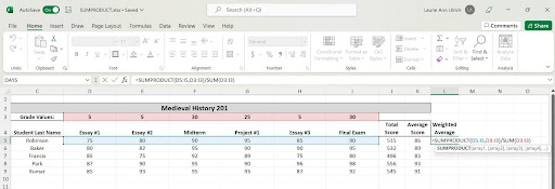
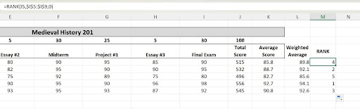
So, using our grades for the students in the Medieval History 201 course, we can weight the average score per student based on the value of each grade earned by each student. Each essay, project, and exam has a different value across the entire course, as shown in row 3 (cells D3 through I3), so weighting the average to reflect the value of each grade given to the students makes the weighted averages more valuable. Why? Because presumably, the grades that are “worth more” – reflective of a greater percentage of the total grade for the course – are the ones to which the students would devote more time and energy.
RANK-ing Your Data
Rank is a tried-and-true Excel function, essential for data analysis. It lets you show how various values in your data rank, in ascending or descending order – without having to sort the records by any given value in the records. Looking at our Final Exam grades for our 5 students, ranking those scores could be done “by eye” – but if we had 50 students or 500 instead, that wouldn’t be so easy. RANK would be required, in such a case, to put the students in order based on their final exam grade.
The function, as shown in the image here, includes 3 arguments:
=RANK(NUMBER, REF, [ORDER])
TIP - Note that ORDER is optional , as indicated by the square brackets.
Let’s look more closely at the arguments:
- Number is a required argument, and it’s the number you want to rank amongst the others in that field for your records.
- Ref is also required, and it’s all the other values in that same field that you want your record ranked against.
- Order is optional, and determines if the rank values are in ascending or descending order. For example, if you choose Ascending (by not entering anything for this argument), 1 is the highest rank. If you enter a 0, for Descending order, 5 is the highest rank.
That’s a Wrap
There are many more functions that give your data more insight and more perspective – from various COUNT functions that isolate unique or repeated values to VLOOKUP and XLOOKUP, that just as their names indicate, allow you to find very specific data in a sea of words and numbers.
Check Out These Videos for More Information:
- To COUNT how many times a value appears in the data – showing frequency of survey responses, test results, or any value you’re tracking:
