Combining and Filtering Data from More than One Worksheet with Microsoft Excel

Discover how to combine data from two different sources using complex formulas, and then create a dynamic dropdown with this information. Learn how to manipulate data according to specific conditions, filter data, and execute advanced functions such as IFERROR, CHOOSECOLS, LET, VSTACK, and INDEX.

Key Insights

The CHOOSECOLS function can rearrange an array according to a specified order. This can be particularly useful when you need to align data from different sources.
The VSTACK function allows for the vertical stacking of data from multiple sources, creating a comprehensive data set that can be stored in memory.
The LET statement can assign a calculation or range to any variable name, simplifying the reference process in complex formulas.
The FILTER function can filter data based on multiple conditions. By multiplying the conditions together, you can create an AND condition.
The IFERROR function can show a specified value (like “None”) when a formula results in an error, giving a clean output even with invalid inputs.
Applying UNIQUE and SORT functions to a combined data set can create a dynamic dropdown list, which can be further refined by the TOCOL function to ignore blanks.

In this article, we’ll explore some amazing new functions in Excel with practical results.

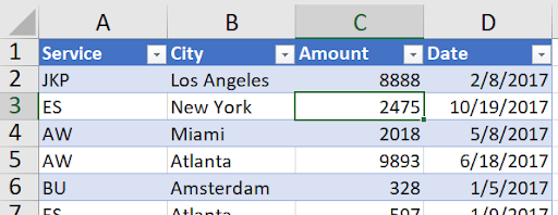
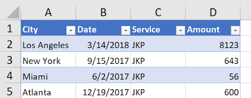
First, let’s look at the data source(s). There are 2 sheets with similar data, but not in the same order:

Source 1:

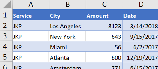
(this continues to row 123). Source 2:

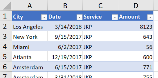
(this continues to row 127).

First, notice the columns aren’t lined up the same way. City, for example, is in column B in the top screenshot and column A in the bottom screenshot. How can you combine this data with a formula before being able to get something like this:

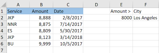
Notice that row 2 comes from the top figure while row 5 comes from the bottom! If the city in f2 is changed, we get:

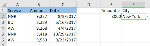
Again, this data comes from both Source1 and Source2. Also, if the figure in E2 is changed, all the data updates as well! Pretty slick.

Time to investigate how this is done in one formula in cell A2!

Here’s the formula:

=IFERROR(CHOOSECOLS(LET(All,VSTACK(Source1!A2:D1000,CHOOSECOLS(Source2!A2:D1000,3,1,4,2)),FILTER(All,(INDEX(All,,3)>E2)*(INDEX(All,,2)=F2))),1,3,4),"None")

Wow. That’s a lot to decipher, and we will. I’ll highlight the section in bold that I’ll be taking apart, starting with this:

=IFERROR(CHOOSECOLS(LET(All,VSTACK(Source1!A2:D1000,CHOOSECOLS(Source2!A2:D1000,3,1,4,2)),FILTER(All,(INDEX(All,,3)>E2)*(INDEX(All,,2)=F2))),1,3,4),"None")

The function CHOOSECOLS takes an array and rearranges it. Source2!A2:D1000 refers to everything except the headers (in row 1), and beyond the last row, just in case the data grows. But the “3,1,4,2” at the end changes this (showing row 1 only for easy reference):

To this:

Now that the data is in the same sequence as Source1’s data, they can be stacked on top of each other:

=IFERROR(CHOOSECOLS(LET(All,VSTACK(Source1!A2:D1000,CHOOSECOLS(Source2!A2:D1000,3,1,4,2)),FILTER(All,(INDEX(All,,3)>E2)*(INDEX(All,,2)=F2))),1,3,4),"None").

This is done in memory, not anywhere on any sheet. This vertical stacking is saved in a variable called “All”:

=IFERROR(CHOOSECOLS(LET(All,VSTACK(Source1!A2:D1000,CHOOSECOLS(Source2!A2:D1000,3,1,4,2)),FILTER(All,(INDEX(All,,3)>E2)*(INDEX(All,,2)=F2))),1,3,4),"None")

The LET statement assigns a calculation or range (the Stacked data in this case) to any variable name and can then be used to easily reference it. The next step is to filter the data using the FILTER statement:

=IFERROR(CHOOSECOLS(LET(All,VSTACK(Source1!A2:D1000,CHOOSECOLS(Source2!A2:D1000,3,1,4,2)),FILTER(All,(INDEX(All,,3)>E2)*(INDEX(All,,2)=F2))),1,3,4),"None")

There are 2 conditions that need to be filtered – the amount needs to be greater than the value in E2 and the city must equal the value in F2. To do an AND condition in a FILTER function, you need to multiply the conditions together (to do an OR condition, you need to add them together).

The INDEX(All,,3) refers to the 3rd column and the INDE(All,,2) refers to the 2nd.

Next is the outermost CHOOSECOLS:
=IFERROR(CHOOSECOLS(LET(All,VSTACK(Source1!A2:D1000,CHOOSECOLS(Source2!A2:D1000,3,1,4,2)),FILTER(All,(INDEX(All,,3)>E2)*(INDEX(All,,2)=F2))),1,3,4),"None")

There’s no need to show the city in the result, since it would be the same throughout, so the CHOOSECOLS chooses all but the 2nd column, hence the “1,3,4” at the end.

Finally, the IFERROR surrounding it all will show the word “None” if you either enter a number too large or an invalid city:

=IFERROR(CHOOSECOLS(LET(All,VSTACK(Source1!A2:D1000,CHOOSECOLS(Source2!A2:D1000,3,1,4,2)),FILTER(All,(INDEX(All,,3)>E2)*(INDEX(All,,2)=F2))),1,3,4),"None")

This is the bulk of the combining data article, but there was one other thing that is worthy of pointing out. The city is a dropdown:

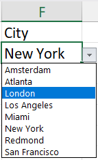
And the source of the dropdown also comes from the combination of the two sheets, Source1 and Source2. This list was in cell H1:

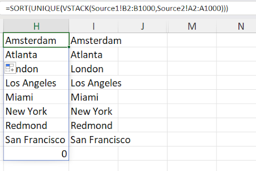
As you can see, column B from Source1 was stacked on top of column A from Source2. Also, applying UNIQUE and SORT gave that dropdown. But notice the 0 in cell H9. This isn’t present in I9, so let’s see how the list in column I was created:

The same formula was surrounded with a TOCOL function using the parameter 1:

=TOCOL(SORT(UNIQUE(VSTACK(Source1!B2:B1000,Source2!A2:A1000))),1)

That parameter is to ignore blanks, which is just what was called for. So the data validation in cell F2 looks like this:

The reference to I1# means to use the Spill range created from the formula in cell I1.

How to Learn Excel